
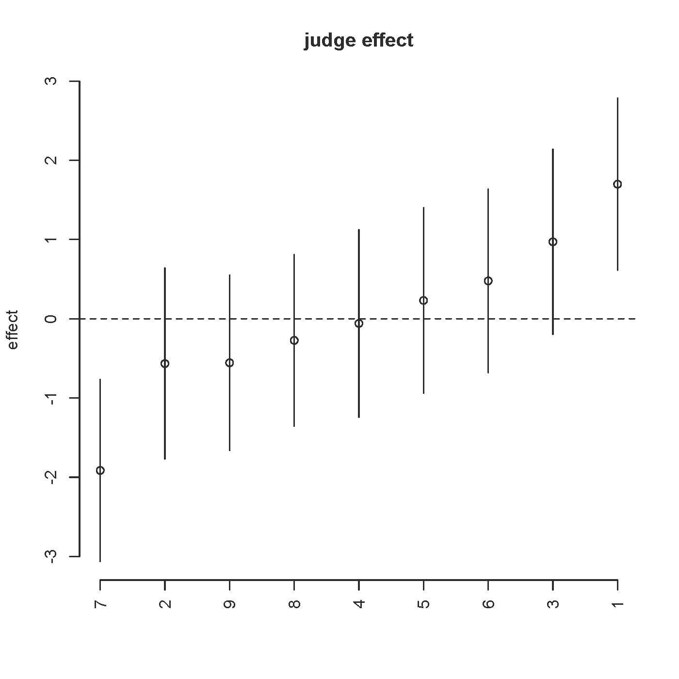
Visualizing random effects when using ordinal package and clmm. This function is based on clmm2 tutorial code and illustrates the effects of each judge taste on evaluating the bitterness of wines.
plot.random <- function(model, random.effect, ylim=NULL, xlab="", main="") {
     rnd <- model$condVar[[random.effect]]
     ci <- model$ranef[[random.effect]] + qnorm(0.975) * sqrt(rnd) %o% c(-1,1)
     ord.re <- order(model$ranef[[random.effect]])
     ci <- ci[order(model$ranef[[random.effect]]), ]
     ylim <- if(is.null(ylim)) range(ci)
     else ylim
     n <- length(model$ranef[[random.effect]])
     plot(1:n, model$ranef[[random.effect]][ord.re], axes=FALSE, ylim=ylim, xlab=xlab, ylab="effect", main=main)
     axis(1, at=1:n, labels=rownames(ci), las=2)
     axis(2)
     for(i in 1:n) {
          segments(i, ci[i,1], i, ci[i,2])
          abline(h=0, lty=2)
     }
}
library("ordinal")
data(wine)
fm2 <- clmm(rating ~ temp + contact + (1|judge), data = wine,Hess = TRUE, nAGQ = 10)
plot.random(fm2, "judge", main="judge effect")
|
|
Visualizing ordinal models is discussed at my previous post.
The data modelled here looks like this:
'data.frame': 72 obs. of 6 variables:
 $ response : num 36 48 47 67 77 60 83 90 17 22 ...
 $ rating   : Ord.factor w/ 5 levels "1"<"2"<"3"<"4"<..: 2 3 3 4 4 4 5 5 1 2 ...
 $ temp     : Factor w/ 2 levels "cold","warm": 1 1 1 1 2 2 2 2 1 1 ...
 $ contact  : Factor w/ 2 levels "no","yes": 1 1 2 2 1 1 2 2 1 1 ...
 $ bottle   : Factor w/ 8 levels "1","2","3","4",..: 1 2 3 4 5 6 7 8 1 2 ...
 $ judge    : Factor w/ 9 levels "1","2","3","4",..: 1 1 1 1 1 1 1 1 2 2 ...
    response rating temp contact bottle judge
1   36        2     cold no      1      1
2   48        3     cold no      2      1
3   47        3     cold yes     3      1
...
